Introduction to Linear Regression
=
Introduction
Welcome to an Introduction to Linear Regression! This tutorial is largely adapted from a similar workshop I hosted while I was an officer at Data Science UCSB. However, in the interest of simplicity, I trimmed much of the material and modified many explanations.
This guide is intended to introduce the principles behind regression, and present linear regression from a data science angle. I intend this largely for beginners who are new to the field, but have some exposure with freshman-level math (e.g. linear algebra).
Prerequisites
I assume that you are comfortable with the following
- Technology
- Python
- NumPy, Pandas
- Mathematics
- Linear Algebra
- Vectors, matrices, linear systems, norms (length/magnitude)
- Linear Algebra
For the most part, I abstracted away the statistical theory and inference behind linear regression. However, I recognize that doing so misses a large part of the story, especially when it comes to interpretability. I intend to write a follow-up guide with these details included.
Data
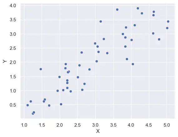
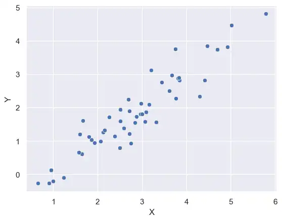
For ease, I will be using simulated data in all my examples.
=
One may object that using simulated data not only begs the question, but also fails to demonstrate applicability. While I agree, finding data compatible with linear regression is incredibly easy. Furthermore, linear regression is so incredibly fundamental that its applicability is not something that needs to be demonstrated.
What is Regression?
Say we're interested in modeling a relationship between a reponse $Y$, and a bunch of explanatory variables $X_1, \dots, X_p$. For example, we may be interested in finding a relationship between
- $Y = $ Average traffic accidents in a day
- $X_1 = $ Average temperature, $X_2 = $ Day of week, $X_3 = $ Month of year
To write this down mathematically, we are trying to find a function $f$ such that
$$ Y = f(X_1, \dots, X_p) + \epsilon $$
Where $\epsilon$ represents an error term. The process of finding such a $f$ that minimizes the error is called1 regression.
1: This isn't always true. Regression is really about finding the "best possible" function, where "best possible" is defined in a clear and tractable way. For our purposes though, let's stick with this framework of minimizing error.
A Problem with Regression
While the problem I outlined above may seem straightforward to solve, it's really vague and broad. For instance, consider the following function $$ f(X_1, \dots, X_p) = \begin{cases} 0 &\text{if we have never seen } X_1, \dots, X_p \\ Y &\text{if we have seen } X_1, \dots, X_p \end{cases} $$
In plain English
Output the answer if we know it. Otherwise, output 0.
It shouldn't be hard to see why this function is a terrible idea. However, as far as the math is concerned, this is the best possible fit for our data. After all, there's no way to know how wrong we are on stuff we've never seen before.
To prevent ridiculous solutions like this, we limit ourselves to a certain class of functions. For example, we might say that
- We are only allowed to consider functions of the form $f(x) = \alpha \sin(x)$ for some constant $\alpha \in \mathbb{R}$
- We are only allowed to consider functions that satisfy the differential equation $f'(x) = x f(x)$.
- We are only allowed to consider the following list
- $x^2 / y$
- $\log(x) + y$
- $y^x$
We can define our class of functions however we want. Above, we explicitly write down the functional form as in (1), write down a condition as in (2), or specify a list as in (3). The class of functions we consider depends heavily on the problem at hand, such as how many inputs there are, and other domain-specific constraints.
Why do we do this? Aside from filtering out dumb solutions, the problem becomes much more tractable.
Linear Regression
When we say linear regression, we are restricting ourselves to the class of linear functions2. That is, we say that $$ Y = \beta_0 + \beta_1 X_1 + \dots + \beta_p X_p + \epsilon $$ And the problem now amounts to finding the coefficients $\vec{\beta} = \left( \beta_0, \dots, \beta_p \right)$ such that $\epsilon$ is as small as possible.
2: Actually, linear regression just means we have a linear function in terms of our coefficients. That is, $Y$ is a linear combination of $\beta_0, \dots, \beta_p$.
The Setup
Up until here, I've been writing everything as a simple equation, but in truth we really have a system of equations. We have a list of response data $(y_1, \dots, y_n)$. For each response $y_i$, we have some corresponding explanatory data $(x_{i1}, \dots, x_{ip})$. This leads us to the system of equations
$$ \begin{align*} y_1 &= \beta_0 + \beta_1 x_{11} + \beta_2 x_{12} + \dots + \beta_p x_{1p} + ϵ_1 \\ y_2 &= \beta_0 + \beta_1 x_{21} + \beta_2 x_{22} + \dots + \beta_p x_{2p} + ϵ_2 \\ &\vdots \\ y_n &= \beta_0 + \beta_1 x_{n1} + \beta_2 x_{n2} + \dots + \beta_p x_{np} + ϵ_n \\ \end{align*} $$
Rewriting this in terms of matrices
$$ \begin{align*} \begin{bmatrix} y_1 \\ y_2 \\ \vdots \\ y_n \end{bmatrix} &= \begin{bmatrix} 1 & x_{11} & x_{12} & \dots & x_{1p} \\ 1 & x_{21} & x_{22} & \dots & x_{2p} \\ \vdots & \vdots & \vdots & \ddots & \vdots \\ 1 & x_{n1} & x_{n2} & \dots & x_{np} \\ \end{bmatrix} \begin{bmatrix} \beta_0 \\ \beta_1 \\ \beta_2 \\ \vdots \\ \beta_p \end{bmatrix} + \begin{bmatrix} \epsilon_1 \\ \epsilon_2 \\ \vdots \\ \epsilon_n \end{bmatrix} \\ &\\ \iff \mathbf{Y} &= \mathbf{X}\vec{\beta} + E \\ \iff \mathbf{Y} &= \hat{\mathbf{Y}} + E \end{align*} $$
Note that
- $\mathbf{Y} = (y_1, \dots, y_n)$ is the vector of true values, $\hat{\mathbf{Y}} = (\hat{y}_1, \dots, \hat{y}_n)$ is the vector of predicted values, and $E = ( \epsilon_1, \dots, \epsilon_n )$ is the error vector.
- Our predictions depend entirely on our coefficients $\vec{\beta}$, i.e. $\hat{\mathbf{Y}} = \mathbf{X}\vec{\beta}$.
Finding our Coefficients
Ultimately, our goal is to make our predictions $\hat{\mathbf{Y}}$ as close to the truth $\mathbf{Y}$ as possible. In other words, we want to choose our coefficients $\vec{\beta}$ such that we minimize the error vector $E = \mathbf{Y} - \hat{\mathbf{Y}}$.
However, there's some nuance here. What does it mean to "minimize the error vector"? Another way to pose this issue is
How do we measure a vector?
The Least Squares Approach
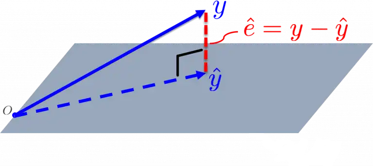
The least squares approach tells us that we should measure the error vector using its magnitude. That is, we "minimize the error vector" by making $||E||$ as small as possible.
Why? Because doing so minimizes the distance between $\mathbf{Y}$ and $\hat{\mathbf{Y}}$.
We call this the least squares approach because minimizing $||E||$ is the same as minimizing its square, $||E||^{2}$, and $$ ||E||^{2} = (\epsilon_1)^2 + \dots + (\epsilon_n)^2 $$
So we're really minimizing the sum of squared errors. Using a bit of calculus, it's rather easy to figure out what this optimal $\vec{\beta}$ is. I leave this detail aside since knowing the exact formula is unimportant for understanding.
Examples
The math here has been rather dense, so let's bring ourselves back into the real-world and construct some models. All the models that follow are based on the data presented at the start of this guide.
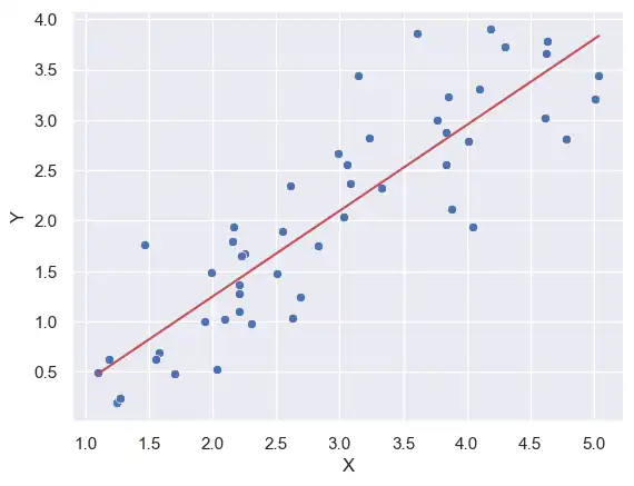
Line of Best Fit
We use the model
$$ \begin{align*} &Y = \beta_0 + \beta_1 X + \epsilon \\ \iff &\hat{Y} = \beta_0 + \beta_1 X \end{align*} $$
=
=
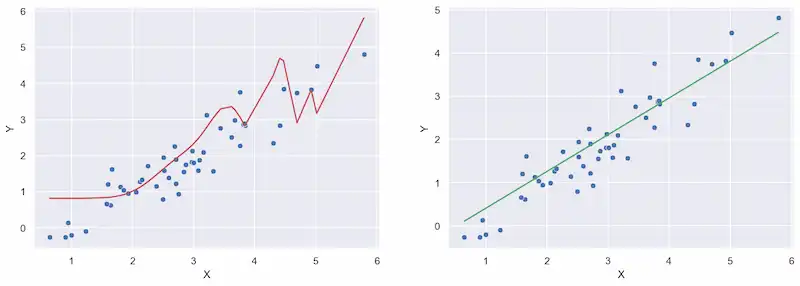
Y = -0.46 + 0.85 X
Polynomial Regression
Rather than finding a line of best fit, say we instead want to use $$ Y = \beta_0 + \beta_1 X + \dots + \beta_k X^k + \epsilon $$ That is, fit a $k$-degree polynomial instead of a line. After all, we know $X$, so finding powers of $X$ is an easy task. This may not seem linear, but it is. See footnote b for a brief comment why.
For our example, we will use $k=25$. That is, fit a 25 degree polynomial.
=
# transforms the data for us.
# include_bias = False since linear regression includes it by default
=
=
, =
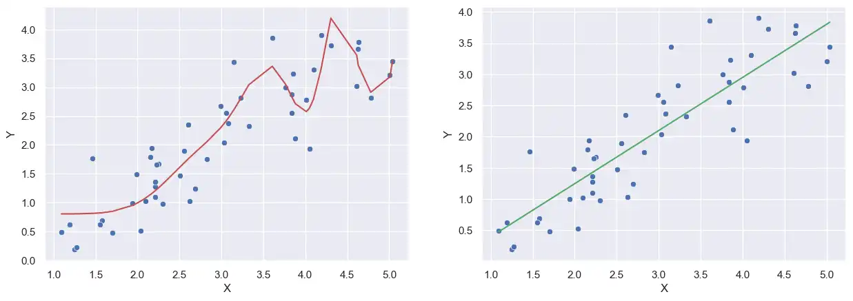
The Problem of Overfitting
Let me draw your attention to the two models above: the polynomial model (red), and the linear model (green).
To an untrained eye, it seems like the polynomial model is performing better than the linear model. However, let's suppose we receive more data.
=
Note that this data came from the exact same source as the original data. Now, to compare our models over this new, unseen data
=
=
=
# filter out values that are too large
= + 1
= - 1
, =
It's fairly clear that the polynomial models does a rather poor job at predicting the new data, especially on the tails. (It's not obvious in the picture, but the right-most point has a prediction in the billions.) While it felt like the polynomial model did a good job with the original data, it does a poor job with everything else.
This phenomenon is called overfitting. Overfitting means that the model fits its training data too well, to the point that it's all but useless for outside data. In other words, we dug ourselves into a situation where the model is only telling us what we already know, and nothing more.
Model Evaluation
While we may know how to train models, we need some criteria by which to evaluate them. After all, how do we know if our model is good? This is especially important in order to identify overfitting. Fortunately, there are many tools available to us at our disposal.
Train-Test Split
As a general rule of thumb, you should always partition your data into two categories: training data and testing data. As the names suggest, the training data is used to find coefficients, while the testing data is used to evaluate generalizability. A common ratio is 75% train and 25% test, though this is completely arbitrary (in this article, we used a 50/50 ratio).
Why do we do this? To test two things
- To check if our model is overfitting the data.
- To see how well our model generalizes to unseen data.
A good model should not only have satisfactory evaluations across both datasets, it should also have very similar evaluations. Otherwise, there's a clear sign that some form of overfitting is taking place.
There are many packages that will do this partitioning for you. Scikit-learn has one that works very well.
$R^2$ Score
The $R^2$ score is a measurement of how well explanatory variance predicts the response variance. Setting $\bar{y}$ as the average of the responses, $R^2$ is defined as $$ \begin{align} R^2 &= \frac{\sum_{i=1}^{n} (\hat{y}_i - \bar{y})^2}{\sum_{i=1}^{n} (y_i - \bar{y})^2} \\ \nonumber \\ &\overset{(!)}{=} 1 - \frac{\sum_{i=1}^{n} (y_i - \hat{y}_i)^2}{\sum_{i=1}^{n} (y_i - \bar{y})^2} \end{align} $$ (1) gives us a clear interpretation of $R^2$ as a ratio of variances. More specifically, the numerator is proportional to the variance of the predictions, while the denominator is proportional to the variance of the response variables. In essence, $R^2$ tells us the amount of response variance explained by the predictions.
(2) is how $R^2$ is computed in many packages, including scikit-learn. However, note that the equality between (1) and (2) is only true over the training data. It is not true in general. (2) is preferred because it's more intuitive to write a metric in terms of error3.
3: Note that the numerator in (2) is precisely $||E||^2$.
As we can see, the polynomial model is performing terribly, achieving a score well-below 0. Since $R^2$ represents a ratio, anything below 0 indicates a serious misfit4.
However, there is much more about $R^2$
- It's mainly useful for evaluating performance on your training data, as interpreting it as a ratio between variances relies on this fact. Evaluating it on outside data loses this interpretation, and thus much its value.
- The attentive reader will note that we did precisely this in the above example.
- It has very questionable efficacy, as "explained variance" is not always a desirable outcome. Good models can have low $R^2$, and terrible models can have high $R^2$.
- In fact, high $R^2$ ($>0.95$) is a good sign of overfitting.
- $R^2$ says nothing more beyond what's outlined above. It depends on many different things, and using it for model selection is very dubious.
This stack exchange answer goes into much more detail. However, there is a reason why $R^2$ still remains a very popular metric. As with many statistics, it's useful but dangerous.
4: Intuitively, negative $R^2$ is only possible if the variance of the predictions is greater than the variance of the response data. In other words, if our predictions create more variability than exists.
Mean Squared Error
The mean squared error is the amount of squared error we can expect in a typical prediction. It is given by5 $$ \mathrm{MSE} = \frac{||E||^2}{n} $$ Which is, quite literally, the average squared error. This is precisely the quantity we minimized when computing our coefficients, suitably standardized by number of datapoints.
One big pitfall of mean squared error is its sensitivity to outliers. This comes from the fact that $\mathrm{big}^2 = \mathrm{bigger}$. In fact, we see this behavior above, since one single datapoint is drastically inflating the MSE for the polynomial model.
It's also important to note the units of MSE, as it's given in units of $Y^2$ rather than $Y$. As a result, interpreting this as a quantity can be rather difficult.
However, in spite of its pitfalls, note that everything in this blog revolves around MSE. After all, when we use least squares, we are defining "best coefficients" in terms of squared error. As before, a useful but dangerous statistic.
5: In statistics literature, a more common definition is $\frac{||E||^2}{n - p - 1}$, which is related to Bessel's correction.
Other Useful Metrics
Going over every evaluation metric available is simply not a good use of our time. However, know that there are many different metrics, each with their own purpose. Which one you use depends entirely on your application.
Here's some more worth checking out.
Conclusion
All this just about summarizes an overview into linear regression. Yet, there's a much bigger world I have not mentioned whatsoever. Namely, alternatives to least squares, as well as the statistical inference and interpretability behind linear regression. I intend to write future tutorials covering these topics, particularly regularization and a statistical-based overview.
Acknowledgements
The projection image found under "The Least Squares Approach" section was adapted from Observation Theory: Estimating the Unknown by TU Delft OpenCourseWare, licensed under CC BY-NC-SA 4.0.