Introduction

Welcome to my introduction on probability theory! This guide is largely meant for those with some exposure to rigorous mathematics. Indeed, as will quickly become apparent, everything here leans far closer to mathematics rather than statistics.

There is good reason for doing so. Probability in and of itself lacks a universal interpretation. Its precise meaning changes with who you ask. So instead of discussing one specific application or meaning, my goal is to present a general theory encompassing everything.

To this end, I must stress the importance of withholding prior conceptions of probability. The best approach, in my opinion, is to simply understand the theory not as something with intrinsic meaning, but as a framework for uncertainty¹.

1: Even then, there are many applications of probability that have nothing to do with uncertainty.

Prerequisites

Familiarity with set theory and discrete mathematics is necessary. Notation such as $x \in A$, $f: A \to B$, and $f^{-1} (E)$ should read fluently to you. Otherwise, you will have a very difficult time understanding this tutorial.

I intend to approach probability theory from a measure-theoretic framework. In my opinion, measure theory is the most natural definition of probability. That said, I recognize such a treatment is difficult for the typical reader, especially those without a background in mathematics, let alone measure theory. As such, I will do my best to reduce difficult details. Nevertheless, familiarity with real analysis may be helpful, though certainly not necessary.

What Is Probability?

As I hoped to communicate in the introduction, probability has no universally agreed meaning. To see why, let's walk through a simple example.

Suppose I'm tossing a coin.

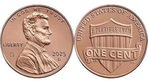
When tossing the coin, there are one of two possibilities. Either it lands with the heads side facing up (heads), or the tails side facing up (tails). Yet without precise knowledge of physical details, such as the strength and direction of the toss, it is impossible to deduce the result with absolute certainty.

However, it's wrong to say we are ignorant. We know the result will be one of heads or tails, both equally likely. How do we describe such uncertainty without admitting total ignorance?

The role of probability is to quantify such uncertainty. Yet the means of doing so brings nuance. To outline² a few interpretations.

1. A frequentist will argue that we should describe uncertainty with long-term frequency. In this case, the probability of heads represents the proportion of tosses resulting in heads as we perform more and more outcomes. Ultimately, this comes out to 50%.
2. A Bayesian will argue that we should describe uncertainty with subjective belief. In this case, the probability of heads represents my reasonable expectation that heads will appear. Most people agree this should be 50%.
3. A propensitist will argue that we should describe uncertainty with physical tendencies. In this case, the probability of heads represents the natural tendency of a coin to land on heads. By symmetry of a coin, this is half, i.e. 50%.
4. An information theorist will argue that we should describe uncertainty with informativeness. If an event carries a lot of information, it must be rare and thus have low probability. In this case, the probability of heads represents how informative it is to see heads. Due to carrying equal³ information as tails, the probability is 50%.

As I hope these examples illustrate, asking what probability means opens much room for debate. While there's overlap among these interpretations, they are ultimately distinct schools of thought with room for disagreement.

In spite of these differences, there is one agreement among all four of them. The probability of heads is 50%, or $\mathbb{P}(\textrm{Heads}) = 0.5$. My goal is to outline this unifying mathematical theory.

2: Keep in mind that these examples should not be taken as wholly accurate representatives of their school of thought.

3: Explaining why requires me to define "information". That's for a different blog.

The Fundamentals

Outcomes and Events

Before we introduce probability, we must first define what probability measures.

To illustrate with an example, suppose I am rolling a six sided die.

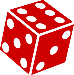
The possible outcomes are 1–6, therefore $\Omega = \{ 1, 2, \dots, 6 \}$ is the sample space. A possible event is rolling an even number, which corresponds to $E_1 = \{ 2, 4, 6 \}$. Another event is nothing, i.e. $E_2 = \varnothing$, and its contrary is something, i.e. $E_3 = \Omega$.

Rolling a six is also an event, $E_4 = \{ 6 \}$. $E_4$ should not be confused with the outcome $\omega = 6$. The difference is subtle, yet simple. $E_4 \subseteq \Omega$ while $\omega \in \Omega$.

With outcomes and events mostly defined, we can now start asking ourselves about collections of events.

4: "Random" is left unaddressed. Indeed, we only assume it exists in some capacity. The precise meaning is left to the aforementioned schools of thought to figure out, and is otherwise unimportant to us.

$\sigma$-algebra

The introduction of Greek⁵ letters may seem intimidating. Nonetheless, I promise that $\sigma$-algebras follows naturally from the previous section.

$\sigma$-algebras encode the basic principles of deductive reasoning. Intuitively, a $\sigma$-algebra captures all the possible events one can deduce with a certain amount of knowledge. To see why, let's translate each property into plain language

1. By definition of a random trial, it must always have an outcome. Therefore, we know $\Omega$ must happen. Hence, we can always deduce it, as uninteresting as it may be.
2. If we know whether $E$ happened, we can say whether its contrary $E^c$ happened. They're mutually exclusive :)
   • A consequence of this and (1) is that $\Omega^c = \varnothing \in \Sigma$. Which logically makes sense. We always know nothing didn't happen.
3. If we have a countable collection of events $E_1, E_2, \dots$, knowing whether each $E_i$ happened, then we can say whether its union $\cup_{i=1}^{\infty} E_i$ happened. Note that unions are essentially OR statements, i.e. $A \cup B$ is the same as $A \textrm{ or } B$.
   • We allow the possibility of infinity for the most flexibility. Besides, having infinitely many outcomes isn't that shocking. Suppose my random trial is the number of attempts needed to throw a basketball into the hoop from across the court. Let $E_1 = \{ 1 \}, E_2 = \{ 2 \}, \dots, E_i = \{ i \}, \dots$
   • However, we must emphasize countable. In uncountable settings, "unions are essentially OR statements" is no longer true.
4. In a similar vein as (3), intersections are essentially AND statements, i.e. $A \cap B$ is the same as $A \textrm{ and } B$.

It will be easy to see the usefulness of these properties with an example.

There's a little more nuance with these examples that involve conditional probabilities. Nonetheless, these examples perfectly illustrate how $\sigma$-algebras encode information.

5: For those curious, the $\sigma$ in $\sigma$-algebra means "countable". $\sigma$ comes from the German word "summe", sum, referring to the fact that $\sigma$-algebras are closed under countable unions, essentially sums of sets.

Probability

A Probability Measure

With $\sigma$-algebras out of the way, we may now define probability.

As before, with a bit of unpacking, the daunting becomes simple.

1. The probability of something happening is 1 (100%).
2. If a collection of events is disjoint, i.e. have no outcomes in common, then the probability of their union is the sum of their probabilities.
   • Intuitively, this property comes from the addition principle.
   • The extension to countable collections rather than finite collections is mostly a convenience to enable work in infinite $\Omega$, such as $\mathbb{N}$ or $\mathbb{R}$.

There's an enormous subtlety with this definition that deserves attention. Note that $\mathbb{P}$ only accepts members of $\Sigma$ as input, not arbitrary subsets of $\Omega$. While seemingly strange, there may be sets of outcomes we do not want to assign numbers to. An example will be given shortly.

Nevertheless, you might ask why we need to define probability measures over $\sigma$-algebras. The true reason is that it's a technical necessity, the details of which come from measure theory. However, at risk of oversimplifying, there's a simple reason why we need to work with $\sigma$-algebras.

One can think of probabilities as a generalization of truth values. Rather than declaring something to be true always, we may declare it to be true with some degree of confidence, à la Bayesianism, or true in some percentage of circumstances, à la frequentism. Regardless of how you decide to make sense of probability, you need to define it in such a way that respects the logic of truth values. The most basic way of doing so is a $\sigma$-algebra, namely a system that encodes the rules of NOT, OR, AND.

Alternatively, here's a geometric explanation from Wikipedia.

$\sigma$-algebras are designed to capture our intuitive ideas about how sizes combine: if there is a well-defined probability that an event occurs, there should be a well-defined probability that it does not occur (closure under complements); if several sets have a well-defined size, so should their combination (countable unions); if several events have a well-defined probability of occurring, so should the event where they all occur simultaneously (countable intersections).

6: We call probability a measure because it, quite literally, assigns numbers to events. In other words, probability measures events.

Spaces and Events (again)

With these, we may now properly define a probability space, and consequentially, an event.

Probability spaces are typically the object of interest. We define the set of possible outcomes ($\Omega$), all events we would like to assign probabilities to ($\Sigma$), and the probability itself ($\mathbb{P}$).

It may be difficult to understand the notation, so let us walk through the die example once more.

7: There's also another reason, although it is well-beyond the scope of this tutorial. If $\Omega = [0, 1]$, it is possible to construct a set that has no meaningful notion of probability, rendering $\Sigma = 2^{[0, 1]}$ impossible. Such counterintuitive examples are only possible in uncountable settings, of course.

Independence

Oftentimes, we are interested in how events relate to each other through probabilities. One of the most useful properties is independence.

In a similar vein how $\mathbb{P} \left( \cup_{i=1}^{\infty} E_i \right) = \sum_{i=1}^{\infty} \mathbb{P}(E_i)$ comes from the addition principle, independence comes from the multiplication principle. As long as $A$ and $B$ don't relate to each other, counting all the possibilities of both is the same as multiplying their number of outcomes together.

Let us now illustrate an example of independence and non-independence.

tip

Example: Non-Independence

Suppose we are still flipping two coins. However, instead of flipping the same coin twice, we decide to use a biased coin for the second flip. Specifically

• If the first result is heads, use a coin that comes up heads 75% of the time, and tails 25% of the time.
• If the first result is tails, use a coin that comes up heads 40% of the time, and tails 60% of the time.

In other words, we bias the second result towards the first, albeit unequally.

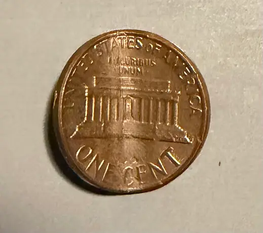
As before, we still have $\Omega = \{ HH, HT, TH, TT \}$ and $\Sigma = 2^\Omega$. However, instead of $\mathbb{P}$, we will use the probability measure

$$ \begin{aligned} &\mathbb{Q}(E) = \tfrac{3}{8} 𝟙_E (HH) + \tfrac{1}{8} 𝟙_E (HT) + \tfrac{1}{5} 𝟙_E (TH) + \tfrac{3}{10} 𝟙_E (TT) \\ \\ &\textrm{where} \quad 𝟙_E (x) = \begin{cases} 1 &\textrm{if } x \in E \\ 0 &\textrm{if } x \notin E \end{cases} \end{aligned} $$

We use $\mathbb{Q}$ to emphasize the difference from $\mathbb{P}$. Now consider the events $A$ and $B$ from the prior section. We have

$$ \begin{aligned} \mathbb{Q}(A) &= \mathbb{Q}\left( \{ HH, TT \} \right) \\ &= \tfrac{27}{40} \\ \mathbb{Q}(B) &= \mathbb{Q}\left( \{ HH, HT \} \right) \\ &= \tfrac{1}{2} \\ \mathbb{Q}(A \cap B) &= \mathbb{Q}\left( \{ HH \} \right) \\ &= \tfrac{3}{8} \end{aligned} $$

So it is clear that $\mathbb{Q}(A \cap B) \neq \mathbb{Q}(A) \mathbb{Q}(B)$.

The important takeaway⁸ of these examples is that independence is a property of probability measures, not of the events or the $\sigma$-algebra. $A$ and $B$ are independent under $\mathbb{P}$, but not under $\mathbb{Q}$. Wiggling around the numbers in $\mathbb{Q}$ is what broke independence.

In practical terms, my point is to highlight the centrality of probability in our model. The probability measure encodes the physical process. $\Omega$ and $\Sigma$ do no such thing.

8: Another takeaway, though not explicitly communicated here, is the usefulness of changing a measure. It's a clever way to simplify the relationship between events when direct computation is too difficult. This is exactly the approach taken with risk-neutral pricing in mathematical finance, for instance, wherein the real-world measure governing markets is replaced with an idealized measure. All that's needed is a means by which to translate between the two measures.

Random Variables

The final, and arguably most important, topic of this tutorial is random variables. Virtually all statistics, and applications of probability more broadly, come in the form of random variables.

Quantification of Processes

While many of my examples were numeric, in practice many probability spaces lack any sort of mathematical structure. For example, common probability spaces include

1. Opinions of humans
2. States of ecosystems
3. Securities in financial markets
4. Outcomes of clinical trials
5. Physical systems

Working with these directly is ugly. Besides, writing them down explicitly is usually impractical or impossible. Aside from requiring information possessed only by the omniscient, we typically care about one particular aspect of the probability space, and nothing more. All this to say, how can we go about modeling only the things we care about?

Simplifying probability spaces is the goal of random variables. In essence, they are a quantification of a random trial.

The precise meaning of $\mathcal{F}$ is complicated. We will defer a proper explanation to the next section. For now, we can think of $\mathcal{F}$ as a quantification of $\Sigma$. Rather than represent events with non-mathematical objects from $\Omega$, we represent it with collections of numbers. In other words, $\Sigma$ uses sets of opinions, living things, financial securities, etc., while $\mathcal{F}$ uses sets of numbers. The latter being far easier to work with, of course.

What is the link between $\Sigma$ and $\mathcal{F}$? The random variable $X$. The definition says so: for any event that occurs in $\mathcal{F}$, we can find a corresponding event that caused it in $\Sigma$ through $X$. Put differently, a random variable is a function that translates events from an abstract probability space into concrete numbers. The important detail, of course, is that $X$ respects and preserves the structure between $\Sigma$ and $\mathcal{F}$.

By far the densest part of this tutorial, so let us walk through an example.

The last point about "efficiency" comes back to interpreting $\sigma$-algebras as information. The most "efficient" $\sigma$-algebra for $X$ represents the minimum amount of information needed in order to predict $X$ with absolute certainty. In this case, if we know whether the roll is even, which is precisely what $\{ \varnothing, \{ 1, 3, 5 \}, \{ 2, 4, 6 \}, \Omega \}$ represents, we can say whether $X$ is 0 or 1. Anything more is redundant.

This also reveals a subtle point. If we take $\Sigma = 2^\Omega$, then any definition of $X$ will be a random variable, regardless of what $S$ and $\mathcal{F}$ may be. After all, there's no way $X$'s pre-images can fall outside $2^\Omega$. So why even bother with the condition on $X$'s pre-images?

Herein lies the importance of $\Sigma$. If we were to use $\Sigma = \{ \varnothing, \{ 1, 3, 5 \}, \{ 2, 4, 6 \}, \Omega \}$, then it's no longer true that any $X$ will work across all possible $S$ and $\mathcal{F}$, i.e. quantifications of our probability space. For instance, set $S = \Omega$, $\mathcal{F} = 2^S$ and take $X(\omega) = \omega$.

As we discussed in a prior example, using the above $\Sigma$ instead of $2^\Omega$ corresponds to the scenario where I only care about the parity of the die roll. In essence, $\Sigma$ dictates which subsets we care about, and which ones we don't⁹.

The above discussion also highlights the importance of $\mathcal{F}$, which will be elaborated in the following section.

9: This is coming back to the recurring theme: why model things we don't care about? If I'm interested in everything in the universe, à la $2^\Omega$, then it's quite silly to ask when something is or isn't important. But in the vast majority of problems, accounting for everything is simply a waste of time. The question becomes meaningful, therefore, once I remove things that stop mattering. A reality that happens very quickly in the uncountable setting.

Pushing Probabilities Forward

We have yet to discuss the role of $\mathbb{P}$ alongside random variables. Yet it is this role that makes random variables most useful.

The importance of the above proposition is not obvious at first glance, yet it is what cements random variables at the core of all applications of probability. Not only do random variables quantify events into real numbers, they enable us to bring probability measures defined over ugly and vague objects into the real numbers where it becomes far more simple and tractable.

As always, it will help to walk through an example.

We can now properly interpret $\mathcal{F}$. It represents the set of all collections of numbers which we want to have a meaningful notion of probability. Generally, this should be as large as possible in order to enable the most flexibility. Of course, making it too large can run into problems, and returns to the original dilemma of balancing model complexity with the things we care about.

Working over $S$

As is done in practice, the proposition implies that it's unnecessary to write down $(\Omega, \Sigma, \mathbb{P})$ directly. Instead, we can define $X$ and $(S, \mathcal{F}, \mathbb{P}^{*})$. $(\Omega, \Sigma, \mathbb{P})$ will exist implicitly, rendering it unnecessary to specify what exactly it is.

The purpose of the above example is to illustrate how probability theory comes into play when modeling real-world scenarios. Truthfully, we really care about the co-domain of our random variable, and at best we only care about what $\Omega$ represents rather than what it actually is. I certainly do not want to go through the trouble of mathematically specifying what the state of the world looks like, let alone a $\sigma$-algebra defined over it.

10: For those curious, this comes from the exponential distribution, though I don't expect you to know what that is.

Conclusion

Much of this blog reads far more technical than most introductions of probability. This is an intentional design choice. I felt dissatisfied with a lot of introductions, as if they're missing the essence of probability. At its core, probability is a neat way to assign numbers to sets. Hence, motivating my presentation of everything with measure theoretic ideas, all the while abstracting the difficult details.

There are plenty of topics I omitted. I made a conscious effort to avoid topics that would normally be classified as "mathematical statistics" and attempted to restrict myself solely to "probability". Nevertheless, the most prominent omissions are expectations, density functions, conditional probability, and stochastic processes. The language of measure theory and $\sigma$-algebras makes discussion of these topics incredibly illuminating. Unfortunately, doing so requires a far deeper mathematical background than what I assumed in the introduction. They are also lengthy and difficult to articulate in a single tutorial. I intend to introduce them in separate guides.

Acknowledgements

1. The American penny image, under "What Is Probability?", is courtesy of the US Mint.
2. The transparent red die image, under "Outcomes and Events", is courtesy of Clipart Panda.
3. The bent penny image, under "Example: Non-Independence", is courtesy of myself. I release it under CC0 1.0 Universal.
   • I produced this image by banging the penny with a hammer alongside my dad, while discussing whether heads or tails is more likely :)