Real Analysis
Introduction
Welcome to my guide on real analysis! This is largely based on my notes from courses I took while an undergraduate math major. My goal is to offer an introduction into the subject that is accessible to non-math majors, while still maintaining mathematical rigor. My plan is to cover some (but not all) of the fundamentals, up until differentiation and integration theory.
Note that this blog is not meant to supplant a course in analysis. A proper introduction into real analysis will require a textbook. I personally recommend Understanding Analysis by Stephen Abbott, or Principles of Mathematical Analysis by Walter Rudin. The former is significantly more accessible, while the latter is a gold standard among undergraduate curriculums.
Prerequisites
Due to the nature of the subject, an above average mathematical maturity is necessary. Familiarity with proofs, set theory, and functions is assumed. Discrete mathematics is typically sufficient for this level of familiarity. These are not details that can be abstracted away, as doing so is antithetical to the goals of real analysis.
What is Real Analysis?
Analysis is tricky for me to define. From Wikipedia:
Real analysis studies the behavior of real numbers, sequences and series of real numbers, and real functions.
Which is true, but not particularly illuminating. Another common definition of analysis is the rigorous undertones of calculus. Perhaps accurate, but still unsatisfying.
To me, real analysis is the study of approximation and limiting behavior. While this is the most simplistic definition, I find it the most intuitive. After all, real analysis is the foundation of much of applied mathematics, which itself is married to approximation.
Why learn analysis?
This is a question I commonly hear from non-math people, especially people going into statistics or data science programs that require analysis as a course.
Truthfully, you don't need analysis for most applications. In fact, many people in industry probably know next-to-nothing about it. In terms of skills useful for a job, analysis is certainly nowhere near the top.
However, broadly labeling analysis as "useless math" is, in my opinion, missing a huge chunk of the story. Analysis is largely what separates graduate-level (i.e. "advanced") work in statistics & data science from undergraduate-level work. This is especially true for research in those fields, as well as research in any field adjacent to applied math (e.g. technology, engineering, etc.).
Anyone at the graduate-level is certainly not using analysis in their day-to-day job, so it's wrong to view analysis as something that offers many direct valuable skills. Rather, it offers a level of intuition and a mathematical foundation that enables understanding of much deeper topics. Many advanced topics become incredibly simple with a sufficient math background, and analysis is absolutely fundamental to those advanced topics.
So why study analysis? Because it makes many things simpler to understand. Especially if you plan on going into a research-oriented role, as the intuitions become necessary rather than a luxury.
The Basics
We begin covering real analysis by first discussing different types of numbers.
Basic Number Systems
Both the natural numbers and integers form the most basic type of number system. In some sense, we can think of them as a starting point.
The rational numbers, denoted $\mathbb{Q}$, are the set of ratios of integers, i.e. $$ \mathbb{Q} = \left\{ \frac{a}{b} : a, b \in \mathbb{Z}, b \neq 0 \right\} $$ Generally, we assume that $a, b$ have no common factors (other than 1).
We call these "rational" numbers because they are a ratio of simpler building blocks, the integers. Indeed, the rational numbers encompass a vast majority of numbers we encounter in everyday life.
Moreover, the rationals have a nice property called density. Between any two rational numbers, there exists another rational. Explicitly, if $r < s$ are both rational, then their average $\frac{r + s}{2}$ is also rational, and $r < \frac{r + s}{2} < s$. In some sense, this means the rationals are "fine", unlike the integers, which are "coarse".
However, despite their ubiquity and density, the rationals do not encompass all numbers.
The number $\sqrt{2}$, defined as the positive number such that $\left(\sqrt{2}\right)^2 = 2$, is not rational.
Rather than showing that the statement "$\sqrt{2}$ is irrational" is true, we show that its contrary, i.e. "$\sqrt{2}$ is rational", must be false. In this way, we demonstrate that the statement must be true since it's impossible for it to be false. While this logical approach seems rather roundabout, it's a quite useful trick to make a problem more tractable.
Now assume the contrary, i.e. that $\sqrt{2}$ is rational. Then by definition of a rational number, we can find two integers $a, b$ such that $$ \sqrt{2} = \frac{a}{b} \quad \textrm{for } a, b \in \mathbb{Z}, b \neq 0 $$
As we noted earlier, we may assume that $a, b$ share no common factors other than 1. This step is crucial.
Rearranging the equation above, we have that $$ 2b^2 = a^2 $$
Therefore, $a^2$ is a multiple of 2, so it is even. Since $a^2$ is even, we must have that $a$ is even. To see this, we note that if $a$ weren't even, then it isn't a multiple of 2, so $a^2$ could not possibly be a multiple of 2.
Thus, since $a$ is even, we can write it as 2 times some integer. Formally, $a = 2k$ for some $k \in \mathbb{Z}$. As a result, we must have that $$ 2b^2 = (2k)^2 = 4k^2 \implies b^2 = 2k^2 $$ So $b^2$ is even, therefore by the same logic as above, $b$ is also even. This means that $a, b$ share a common factor of 2. But we assumed earlier that $a, b$ do not share any factors, other than 1. This is a contradiction, so it's impossible for $\sqrt{2}$ to be rational. Thus, $\sqrt{2}$ is irrational.
This "incompleteness" of $\mathbb{Q}$ motivates the definition of the real numbers.
1: This definition of $\mathbb{N}$ excludes 0, which is a major source of debate among mathematicians. However, this definition of $\mathbb{N}$ is the most common, and natural (ba-dum-tss), in analysis. If needed, we will use $\mathbb{N}_0$ to denote the natural numbers including 0.
2: We use $\mathbb{Z}$ for integers because of the German word "Zahlen", meaning "numbers".
The Real Numbers
A proper definition of the real numbers is incredibly technical, and for this article, quite pedantic. We may instead rely on the following intuitive definition.
The real numbers, denoted $\mathbb{R}$, is the set of all numbers that can be represented with an infinite decimal expansion. E.g. $\sqrt{2} = 1.41421\dots$
It's easy to see that $\mathbb{Q} \subset \mathbb{R}$. Moreover, just like the rationals, the reals have density. If $x < y$ are both real numbers, then their average $\frac{x + y}{2}$ is also real, and $x < \frac{x + y}{2} < y$.
But more importantly, there is a profound relationship between the rationals and the reals.
Between any two real numbers, there exists a rational number.
Explicitly, if $x < y$ are both real, then there exists $r \in \mathbb{Q}$ such that $x < r < y$.
Unfortunately, we have to be a bit more clever than taking the average, since the average of two reals may not be rational.
Unlike before, we will prove this directly by explicitly constructing a rational number satisfying our statement. However, before we may proceed further, there are two crucial observations that we must make
- There is no such thing as a "largest" natural number. In other words, the natural numbers grow to infinity. Formally, $\mathbb{N}$ is unbounded3 from above.
- Similarly, the integers run off to both positive infinity and negative infinity. Formally, $\mathbb{Z}$ is unbounded from below and from above.
Now to prove the theorem, let $x < y$ be any two real numbers. Our goal is to find a rational number between them. First, since the natural numbers are unbounded from above, we can find $n \in \mathbb{N}$ such that $$ n > \frac{1}{y - x} $$
There is no trickery here, we simply take any natural number greater than $\frac{1}{y - x}$ (the reason for this will be clear shortly). Note that since $x < y$, $\frac{1}{y-x} > 0$.
Recall from basic algebra that if $a > b > 0$, then $\frac{1}{a} < \frac{1}{b}$. Therefore, $$ \frac{1}{n} < y - x $$
This gives one half of the rational number we want.
To produce the second half, let $m \in \mathbb{Z}$ be the largest integer such that $m \leq nx$. Since $\mathbb{Z}$ is unbounded from below, such an $m$ exists. Then this tells us that $$ m \leq nx < m + 1 $$ Why the second inequality? Because if it didn't hold, then $m + 1 \leq nx$, meaning $m$ is not the largest integer such that $m \leq nx$. (Recall that adding two integers together gives you another integer.) Therefore, we have $$ \frac{m}{n} \leq x < \frac{m+1}{n} $$
Putting everything together, we have that $$ \begin{aligned} x &< \frac{m + 1}{n} \\ &= \frac{m}{n} + \frac{1}{n} &&\left( \textrm{Splitting the fracion} \right) \\ &\leq x + \frac{1}{n} &&\left( \frac{m}{n} \leq x \right) \\ &< x + (y - x) &&\left( \frac{1}{n} < y - x \right)\\ &= y \end{aligned} $$
Which says precisely that $x < \frac{m + 1}{n} < y$. Thus, $r = \frac{m + 1}{n} \in \mathbb{Q}$ is the desired rational number.
An immediate consequence of this is that every real number can be approximated by a rational number to arbitrary precision. For example, $\sqrt{2}$ can be approximated by the rational number $1.41$ to two decimal places, $1.41421$ to five decimal places, and even $1.41421356237309504880$ to twenty decimal places. For any given error threshold and real number $x$, we can always find a rational number $r$ such that the distance between $x$ and $r$ is less than the error threshold.
At this point, we may begin to ask what the point of the reals are. After all, every real number can be approximated by a rational number. To further motivate this idea of "completeness", we must segue into the concepts of bounds, infimums, and supremums.
3: I technically haven't defined what it means to be "unbounded", though this will be explained in the next section.
The Infimum and Supremum
A major concept in real analysis is the idea of bounds.
Let $M$ be a subset of $\mathbb{R}$. We say that $a$ is an upper bound of $M$ if $$ \textrm{For every } x \in M, \quad x \leq a $$
Similarly, we say that $b$ is a lower bound of $M$ if $$ \textrm{For every } x \in M, \quad x \geq b $$
For instance, let $M = [0, 1)$. Then 2 is an upper bound of $M$, and -1 is a lower bound of $M$.

However, it's not hard to see that we can do better. 1.5 and -0.5 are also upper and lower bounds, respectively. In fact, there are infinitely many upper and lower bounds for $M$.
This motivates the definitions of the supremum and infimum, which are Latin for "above" and "below", respectively.
Let $M$ be a subset of $\mathbb{R}$. The supremum of $M$, denoted $\sup M$, is the least upper bound of $M$. More rigorously, $\sup M$ satisfies
$$ \begin{aligned} &\textrm{(1) For every } x \in M, &&x \leq \sup M \\ &\textrm{(2) For every } \varepsilon > 0, &&\sup M - \varepsilon \textrm{ is not an upper bound of } M \end{aligned} $$
Similarly, the infimum of $M$, denoted $\inf M$, is the greatest lower bound of $M$. More rigorously, $\inf M$ satisfies
$$ \begin{aligned} &\textrm{(I) For every } x \in M, &&x \geq \inf M \\ &\textrm{(II) For every } \varepsilon > 0, &&\inf M + \varepsilon \textrm{ is not a lower bound of } M \end{aligned} $$
While $\varepsilon$ (epsilon) may be any positive real number, we typically think of it as an astronomically tiny number.
Property (1) ensures that the supremum is an upper bound, while property (2) ensures that it is the smallest such upper bound. Intuitively, property (2) says that if we nudge the supremum down by any amount, it will no longer be an upper bound. The same logic applies to the infimum.

In our previous example of $M = [0, 1)$, we have that $\sup M = 1$ and $\inf M = 0$, since for any $\varepsilon > 0$, we can always find numbers in $M$ that are greater than $1-\varepsilon$ and less than $0+\varepsilon$.
Why do we care about the supremum and infimum? Because this is precisely what separates the real numbers from the rational numbers.
If $M$ is a non-empty subset of $\mathbb{R}$ that is bounded above, then $\sup M$ exists and is a unique, real number. We call this the completeness property4 of the real numbers.
While completeness is stated only in terms of the supremum, it's true for the infimum as well. We can simply consider the set $-M = \{ -x : x \in M \}$, and note that $\inf M = -\sup(-M)$.
As we've been alluding to, $\mathbb{Q}$ is not complete. For example, let $$ A = \{ x \in \mathbb{Q} : x^2 < 2 \} $$
Then $A$ is bounded above by 2, a rational number. In fact, there are infinitely many rational upper bounds. However, since $\sup A = \sqrt{2} \notin \mathbb{Q}$, there is no smallest rational upper bound of $A$.
4: No proof is given since this is more of a definition than a proof. In the same way that we built $\mathbb{Q}$ from $\mathbb{Z}$ with division, we can build $\mathbb{R}$ from $\mathbb{Q}$ with supremums (see Dedekind cuts). While you can prove this from first principles, it is incredibly difficult and tedious to do so.
Sequences and Limits
By far the most important concept in analysis is that of sequences and limits.
However, we must first establish a very important inequality.
For all $x, y \in \mathbb{R}$, $$ |x + y| \leq |x| + |y| $$
This says that traveling along a path of length $|x + y|$ is always more efficient than moving along two paths of lengths $|x|$ then $|y|$. While they may be equal when $x$, $y$ are both positive/negative, this becomes an inequality when $x, y$ no longer share a sign.
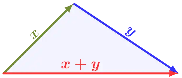
Observe that $$ \begin{aligned} &|x + y| \leq |x| + |y| \\ \iff &(x + y)^2 \leq (|x| + |y|)^2 \\ \iff &x^2 + 2xy + y^2 \leq x^2 + 2|xy| + y^2 \\ \iff &xy \leq |xy| \end{aligned} $$ And the last line is always true since $a \leq |a|$. So the triangle is equivalent to a statement that's always true, therefore the triangle inequality is always true.
Sequences
A sequence $a$ is a function $a: \mathbb{N} \to \mathbb{R}$. We denote the value of the sequence at $n \in \mathbb{N}$ as $a_n = a(n)$.
The notation $\{a_n \}_{n=1}^{N}$ refers to the set $\{a_1, a_2, \dots, a_N\}$. Similarly, $\{ a_n \}_{n=1}^{\infty} = \{a_1, a_2, \dots \}$
Thinking of a sequence as a function is rather technical. Truthfully, a sequence is a list of numbers. For instance, the Fibonacci sequence is given by $$ \{ F_n \}_{n=1}^{\infty} = \{ 1, 1, 2, 3, 5, 8, 13, 21, \dots \} $$
We say that a sequence $a_n$ converges to $a \in \mathbb{R}$ if, for every $\varepsilon > 0$, we can find $N = N(\varepsilon) \in \mathbb{N}$ such that $$ n \geq N \implies |a_n - a| < \varepsilon $$
To denote convergence to $a$, we may write $a_n \to a$ or $\lim\limits_{n \to \infty} a_n = a$.
If a sequence doesn't converge to any real number, we say it diverges.
The notation $N(\varepsilon)$ simply means that $N$ may depend on $\varepsilon$. For example, define the sequence $a_n = \frac{1}{n}$. For any $\varepsilon > 0$, choose $N \in \mathbb{N}$ such that $N > \frac{1}{\varepsilon}$ (possible because $\mathbb{N}$ is unbounded from above). Then we have that $$ n \geq N \implies \left| a_n - 0 \right| = \frac{1}{n} \leq \frac{1}{N} < \varepsilon $$ Which says precisely that $a_n \to 0$.
To give an example of divergence, consider the sequence $b_n = (-1)^{n}$. Then we can enumerate $b_n$ as $\{-1, 1, -1, 1, \dots\} = \{ -1, 1 \}$. Thus, if $b_n \to b$, then either $b = -1$ or $b = 1$.
We first show that $b = 1$ is impossible. By definition of $b_n$, $$ |b_n - 1| = \begin{cases} 2 &\textrm{if $n$ is odd} \\ 0 &\textrm{if $n$ is even} \end{cases} $$
Indeed, if we take $\varepsilon = 0.01$, then we cannot guarantee that $|b_n - 1| < \varepsilon$ for every $n$ sufficiently large. No matter how large we make $N$, we can always find some $n \geq N$ such that $|b_n - 1| \geq \varepsilon$. This says precisely that $b_n$ does not converge to $1$, i.e. $b_n \not\to 1$.
The case for $b = -1$ is identical to above. Therefore, $b_n$ diverges.
Note that there is one minor, but very important, detail I'm glossing over.
If $a_n \to a$, then $a$ is unique. More formally, if $a_n \to a$ and $a_n \to b$, then $a = b$.
This essentially means that our notion of convergence is well-defined, and that sequences may only converge to one number (hence, why the $b_n$ example above failed).
Assume $a_n \to a$ and $a_n \to b$. To prove the statement, we simply need to show that $a = b$. That is, $a_n$ always converges to the same number.
We appeal to the definition of convergence. Pick any $\varepsilon > 0$. Since $a_n \to a$, we can find $N_a \in \mathbb{N}$ such that $$ n \geq N_a \implies |a_n - a| < \frac{\varepsilon}{2} $$
Note that $\frac{\varepsilon}{2}$ is simply just another number. Similarly, since $a_n \to b$, we can find $N_b \in \mathbb{N}$ such that $$ n \geq N_b \implies |a_n - b| < \frac{\varepsilon}{2} $$
We don't know whether $N_a$ and $N_b$ are the same, since $a_n \to a$ and $a_n \to b$ are separate statements. However, since convergence only relies on $n$ being greater than them, it really doesn't matter. Both statements are true as long as $n$ is greater than $N_a$ and $N_b$.
So when $n \geq \max\{ N_a, N_b \}$, we have $$ \begin{aligned} |a - b| &= |(a_n - b) - (a_n - a)| &&\left( \textrm{Adding and subtracting $a_n$} \right) \\ &\leq |a_n - a| + |a_n - b| &&\left( \textrm{Triangle Inequality} \right) \\ &< \frac{\varepsilon}{2} + \frac{\varepsilon}{2} &&\left( \textrm{Both terms less than } \frac{\varepsilon}{2} \right) \\ &= \varepsilon \end{aligned} $$
Note that $|a - b|$ is independent of $n$. Therefore, $|a - b| < \varepsilon$ for any $\varepsilon > 0$.
Since $|a - b|$ is independent of $\varepsilon$, it can be made arbitrarily small while also remaining constant. This is only possible when $|a - b| = 0$. In other words, $a - b = 0 \iff a = b$
Cauchy Sequences
Cauchy sequences, named after famous mathematician Augustin-Louis Cauchy, form an incredibly important class of sequences.
Let $a_n$ be a sequence. We say that $a_n$ is a Cauchy sequence if, for every $\varepsilon > 0$, there exists $N = N(\varepsilon) \in \mathbb{N}$ such that $$ n, m \geq N \implies |a_n - a_m| < \varepsilon $$
Intuitively, a sequence is Cauchy if the terms get arbitrarily close to each other. Convergent sequences have this property.
If $a_n \to a$, then $a_n$ is Cauchy.
Pick any $\varepsilon > 0$. Since $a_n \to a$, we can find $N \in \mathbb{N}$ such that $$ n \geq N \implies |a_n - a| < \frac{\varepsilon}{2} $$
Then for any $m, n \geq N$, we have that $$ \begin{aligned} |a_n - a_m| &= |(a_n - a) - (a_m - a)| &&\left( \textrm{Adding and subtracting } a \right) \\ &\leq |a_n - a| + |a_m - a| &&\left( \textrm{Triangle Inequality} \right) \\ &< \frac{\varepsilon}{2} + \frac{\varepsilon}{2} &&\left( \textrm{Both terms less than } \frac{\varepsilon}{2} \right) \\ &= \varepsilon \end{aligned} $$
Therefore, $m, n \geq N \implies |a_m - a_n| < \varepsilon$, which says precisely that $a_n$ is Cauchy.
Marvelously, Cauchy sequences capture the idea of convergence without invoking convergence. Instead, it relies on the idea of "closeness".
One may ask whether there exists non-convergent Cauchy sequences. The answer is it depends. The answer is also precisely what separates $\mathbb{R}$ from $\mathbb{Q}$.
Let $E$ be a subset of $\mathbb{R}$. We say $E$ is complete5 if every Cauchy sequence in $E$ converges to a point in $E$.
Intuitively, a space is complete if there aren't any "gaps". To be incomplete means that a sequence may approach a hole with nothing in it. As such, $\mathbb{R}$ is complete, while $\mathbb{Q}$ isn't. This is to say that every Cauchy sequence converges in $\mathbb{R}$, but may not converge in $\mathbb{Q}$.
5: We already defined "completeness" using supremums in the prior section. Indeed, "supremum completeness" and "Cauchy completeness" are saying the same thing, though it's not obvious why.
Point-Set Topology
While this section is a bit of a diversion from the prior, point-set topology is fundamental to real analysis. Viewing things under a topological lens often greatly simplifies problems. Moreover, it builds good intuition.
Topology feels rather abstract. However, it is essentially "geometry without distance". Rather than quantifying "closeness" with distance, we quantify "closeness" with open sets.
Open Sets
Before we can define an open set, we must first define a neighborhood.
Let $x \in \mathbb{R}$ and $\varepsilon > 0$. The neighborhood of $x$ with radius $\varepsilon$, denoted $N_\varepsilon (x)$, is defined as $$ N_\varepsilon (x) = \{ y \in \mathbb{R} : |y - x| < \varepsilon \} $$
Note that this is simply the open interval $(x - \varepsilon, x + \varepsilon)$.
Sometimes neighborhoods are called open balls6, as $N_\varepsilon (x)$ is quite literally an open 1-dimensional ball of radius $\varepsilon$ centered at $x$.
Let $U$ be a subset of $\mathbb{R}$. We say that $U$ is open if for every $x \in U$, there exists $\varepsilon > 0$ such that $N_\varepsilon (x) \subseteq U$.
In other words, for every $x \in U$, we can find a neighborhood around $x$ that is entirely contained within $U$.
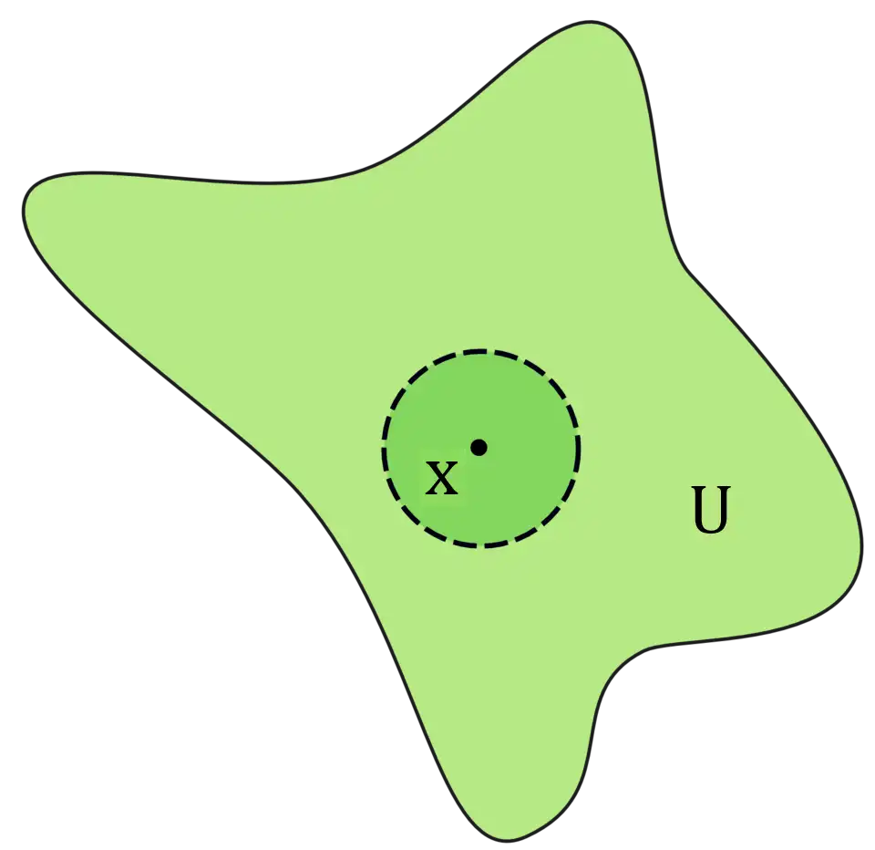
Intuitively, a set is open if every point has "breathing room" in every direction. Points on the boundary do not have this "breathing room", since any neighborhood around them must include points outside the set.
6: The astute reader will notice that the concept of neighborhoods, and by extension open sets, extends to higher dimensions very easily. Indeed, by replacing the absolute value with the Euclidean norm in the definition of neighborhood, we enter the setting for $\mathbb{R}^n$.
Closed Sets
To introduce closed sets, we must first define limit points.
Let $M$ be a subset of $\mathbb{R}$. A point $x \in \mathbb{R}$ is a limit point of $M$ if for every $\varepsilon > 0$, the neighborhood $N_\varepsilon (x)$ contains at least one point of $M$, excluding $x$ itself. More formally,
$$ \textrm{For every } \varepsilon > 0, \quad (N_\varepsilon (x) \setminus \{ x \} ) \cap M \neq \varnothing $$
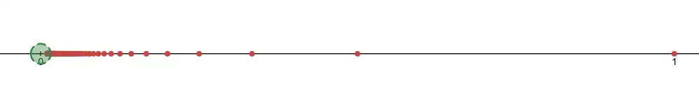
This definition may seem tricky, but the idea is rather simple. Consider the set $$ A = \left\{ \frac{1}{n} : n \in \mathbb{N} \right\} $$ Then 0 is a limit point of $A$, since for any $\varepsilon > 0$, we can find $k \in \mathbb{N}$ such that $\frac{1}{k} < \varepsilon$. Thus, $\frac{1}{k} \in N_\varepsilon (0)$.
Let $C$ be a subset of $\mathbb{R}$. We say that $C$ is closed if it contains all of its limit points. More formally, if $x$ is a limit point of $C$, then $x \in C$.
Closed sets are commonly thought of as sets that contain their boundaries. While not fully accurate, it's helpful intuition, since boundary points are precisely the limit points that are not within the "interior" of the set.
Using the previous example, the set
$$ \left\{ \frac{1}{n} : n \in \mathbb{N} \right\} \cup \{ 0 \} $$
is closed, since it contains its only limit point, 0. Moreover, the interval $[0, 1]$ is closed, since it contains all its limits points (which, coincidentally, is the entire set).
Open and Closed Sets
An important relationship between open and closed sets is that they are complements of each other.
Let $U$ be a subset of $\mathbb{R}$. Then $U$ is open if and only if $U^c$ is closed.
We really have two statements to prove. Namely, that $U \textrm{ open} \implies U^c \textrm{ closed}$ and $U \textrm{ open} \impliedby U^c \textrm{ closed}$
($\implies$): Assume $U$ is open. We have to show that $U^c$ contains all its limit points, so let $x$ be any limit point of $U^c$.
By definition of a limit point, for every $\varepsilon > 0$, the neighborhood $N_\varepsilon (x)$ contains at least one point of $U^c$, excluding $x$ itself. This means that $N_\varepsilon (x) \nsubseteq U$ for every $\varepsilon > 0$. Since $U$ is open, $x \notin U$. Therefore, $x \in U^c$, so $U^c$ contains all its limit points.
(If the explanation for $x \notin U$ didn't make sense, here's an intuitive explanation. Since $U$ is open, every point in $U$ must have "breathing room". We showed that $x$ lacks this "breathing room", so $x$ cannot be in $U$.)
($\impliedby$): Now assume $U^c$ is closed. We have to show that every point in $U$ has "breathing room".
Let $x \in U$. Since $U^c$ is closed, it contains all its limit points, so $x$ is not a limit point of $U^c$. This must mean that we can find some $\varepsilon > 0$ such that $N_\varepsilon (x)$ contains no points of $U^c$. Thus, $N_\varepsilon (x) \subseteq U$. This says precisely that $U$ is open.
Sequences and Topology
At this point, you may be inclined to ask why the topology diversion. After all, there's no obvious connection between the prior discussion and topology.
I'm here to say that they're really the same thing, just viewed under different lenses. Let's revisit the example $$ A = \left\{ \frac{1}{n} : n \in \mathbb{N} \right\} $$
Now define $a_n = \frac{1}{n}$. Then $ \{ a_n \}_{n=1}^{\infty} = A$. We showed that $a_n \to 0$, and that $0$ is the only limit point of $A$. Indeed, these are both saying the same thing. To say $a_n \to 0$ means that $n \geq N \implies |a_n - 0| < \varepsilon$. In other words, if $n \geq N$, the neighborhood $N_\varepsilon (0)$ contains $a_n$.
This observation is formalized with the following theorem
Let $a_n$ be a sequence. Then $a_n \to a$ if and only if every open set $U$ containing $a$ also contains all, but finitely many, elements of $a_n$.
Note that "all, but finitely many" is another way of saying $\textrm{There exists $N$ such that for } n \geq N\dots$
As before, we really have two statements to prove.
($\implies$): Assume $a_n \to a$, and let $U$ be an open set containing $a$. We must show that $U$ contains all, but finitely many, elements of $a_n$.
Since $U$ is open, we may find some $\varepsilon > 0$ such that $N_\varepsilon (a) \subseteq U$. Moreover, since $a_n \to a$, we can find $N$ such that $n \geq N \implies |a_n - a| < \varepsilon$. Then $n \geq N \implies a_n \in N_\varepsilon (a) \subseteq U$, so $U$ contains all, but finitely many, $a_n$.
($\impliedby$): Assume every open set containing $a$ also contains all, but finitely many, elements of $a_n$. We will proceed by contradiction and show that the contrary is impossible.
So assume $a_n \not\to a$. Then we can find $\varepsilon > 0$ such that $|a_n - a| \geq \varepsilon$ for infinitely many $n$. In other words, the open set $N_\varepsilon (a)$ is missing infinitely many $a_n$. Thus, we found an open set containing $a$, yet fails to contain all, but finitely many, $a_n$. This is a contradiction, and hence we must have that $a_n \to a$.
This formalizes topology as "geometry without distance", since convergence is characterized entirely by open sets. In other words, we characterize convergence not by distance, but by membership in certain sets.
Functions and Continuity
Extending all our discussion to functions, and thus making analysis much more applicable beyond sequences.
Usual Notions of Continuity
There are many definitions of continuity, with some being more useful than others. We focus on 3 of them.
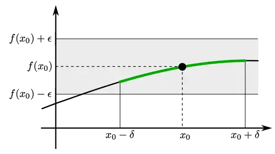
Let $f: X \to \mathbb{R}$ where $X \subseteq \mathbb{R}$. We say $f$ is continuous at $x_0$ if, for every $\varepsilon > 0$, we can find some $\delta = \delta(x_0, \varepsilon) > 0$ such that
$$ y \in X \textrm{ and } |x_0 - y| < \delta \implies |f(x_0) - f(y)| < \varepsilon $$
Note that $\delta = \delta(x_0, \varepsilon)$ means that $\delta$ may depend on both $x_0$ and $\varepsilon$.
Intuively, this definition says the following. For every error-bound $\varepsilon$ of the outputs we impose in the codomain, we can find a corresponding error-bound $\delta$ of the inputs in the domain. In other words, saying that $f$ is continuous at $x_0$ is saying that $f$ preserves "closeness" at $f(x_0)$. Having a tiny bit of error in $x_0$ implies a tiny bit of error in $f(x_0)$ (i.e. no sudden "jumps")
While this definition is good, there is another, and more natural in my opinion, way to think of continuity.
Let $f: X \to \mathbb{R}$ where $X \subseteq \mathbb{R}$. We say $f$ is continuous at $x_0$ if, for every sequence $x_n$ such that $x_n \to x_0$, we have that $f(x_n) \to f(x_0)$. Writing this formally,
$$ x_n \to x_0 \implies f(x_n) \to f(x_0) $$
This definition has an immediate interpretation. If a function is continuous at $x_0$, then it preserves sequences that converge to $x_0$. In other words, a function is continuous if and only if it preserves convergence of sequences.
Naturally, I would not introduce two separate definitions if they weren't saying the same thing.
A function $f: X \to \mathbb{R}$ is $(\varepsilon, \delta)$-continuous at $x_0$ if and only if it is sequentially continuous at $x_0$
($\implies$): Assume $f$ is $(\varepsilon, \delta)$-continuous, and let $\varepsilon > 0$. Take any sequence $x_n$ such that $x_n \to x_0$. We must show that $f(x_n) \to f(x_0)$.
Since $f$ is $(\varepsilon, \delta)$-continuous, we may find a $\delta$ such that $$ |x_0 - y| < \delta \implies |f(x_0) - f(y)| < \varepsilon $$ Since $x_n \to x_0$, we can find $N$ such that $n \geq N \implies |x_n - x_0| < \delta$. Then we have that $n \geq N \implies |f(x_0) - f(x_n)| < \varepsilon$. Hence, $f(x_n) \to f(x_0)$
($\impliedby$): Assume $f$ is sequentially continuous at $x_0$. Similar to the topological convergence proof above, we will proceed by contradiction and show that we can violate the requirement $x_n \to x_0 \implies f(x_n) \to x_0$.
So assume $f$ is not $(\varepsilon, \delta)$-continuous at $x_0$. Then there exists some $\varepsilon > 0$ such that, for every $\delta > 0$ and some $y = y(\delta) \in X$, we have $$ |x_0 - y| < \delta, \textrm{ yet } |f(x_0) - f(y)| \geq \varepsilon $$ Using this fact, we may construct a sequence $x_n$ such that $$ |x_0 - x_n| < \frac{1}{n}, \textrm{ yet } |f(x_0) - f(x_n)| \geq \varepsilon $$ That is, we specify $\delta = \frac{1}{n}$, and set $x_n$ to be some $y$ that satisfies this condition. By construction, we have that $x_n \to x_0$. Yet since $|f(x_0) - f(x_n)| \geq \varepsilon$ for every $n$, we have that $f(x_n) \not\to f(x_0)$. Then $f$ can't be sequentially continuous, which is a contradiction.
Topological Continuity
A more general, and mathematically useful in my opinion, definition of continuity is the topological definition of continuity. This definition motivates many nice generalizations, such as measurable functions.
Let $f: X \to \mathbb{R}$ where $X \subseteq \mathbb{R}$. We say $f$ is continuous if, for every open set $U \subseteq \mathbb{R}$, the pre-image $f^{-1} (U) \subseteq X$ is also open.
There are two important things to note here
- This is a global definition of continuity, whereas the prior two definitions were local definitions (i.e. true at a single point).
- When the domain $X \neq \mathbb{R}$, the definition of "open" changes slightly, though not significantly. Those interested should read this stack exchange.
At first glance, it's not obvious why topological continuity is at all related to previous notions of continuity, especially "closeness". The intuition here is the following.
Understanding topology as "geometry without distance", we interpret open sets as one way to quantify "closeness". When we say that $U \textrm{ open} \implies f^{-1} (U) \textrm{ open}$, we are requiring that any way we decide to quantify closeness in the codomain (namely, through $U$) should correspond to some quantification of closeness in the domain (namely, through $f^{-1} (U)$). In other words, we require that $f$ respects the "closeness" structure of both the domain and codomain.
Another way to see how topological continuity is related is to simply prove that it is equivalent.
Let $f: X \to \mathbb{R}$. Then $f$ is topologically continuous if and only if it is $(\varepsilon, \delta)$-continuous at every point $x_0 \in X$.
($\implies$): Assume $f$ is topologically continuous. Pick any $x_0 \in X$. We must show that $f$ is $(\varepsilon, \delta)$-continuous at $x_0$.
So let $\varepsilon > 0$. Consider the open set $N_\varepsilon (f(x_0))$. By assumption, we have that $$ f^{-1} \left( N_\varepsilon (f(x_0)) \right) \textrm{ is open} $$
Since $x_0 \in f^{-1} \left( N_\varepsilon (f(x_0)) \right)$, we can find some $\delta > 0$ such that $N_\delta (x_0) \subseteq f^{-1} \left( N_\varepsilon (f(x_0)) \right)$. This says precisely that, if $y \in N_\delta (x_0)$, then we have $$ |x_0 - y| < \delta \implies |f(x_0) - f(y)| < \varepsilon $$
Meaning $f$ is $(\varepsilon, \delta)$-continuous at $x_0$.
($\impliedby$): Assume $f$ is $(\varepsilon, \delta)$-continuous at every $x_0 \in X$. For ease, we may rewrite the definition of $(\varepsilon, \delta)$-continuous as follows $$ \begin{aligned} &|x_0 - y| < \delta \implies |f(x_0) - f(y)| < \varepsilon \\ \iff &y \in N_{\delta} (x_0) \implies f(y) \in N_\varepsilon (f(x_0)) \\ \iff &f(N_{\delta} (x_0)) \subseteq N_\varepsilon (f(x_0)) \end{aligned} $$
In other words, being $(\varepsilon, \delta)$-continuous is the same as saying that the image of an open ball is contained in another open ball.
Let $U$ be open, and take any $x_0 \in f^{-1} (U)$. Then $f(x_0) \in U$. Since $U$ is open, we can find $\varepsilon > 0$ such that $N_\varepsilon (f(x_0)) \subseteq U$. Moreover, because $f$ is $(\varepsilon, \delta)$-continuous at $x_0$, we can find some $\delta > 0$ such that $f(N_{\delta} (x_0)) \subseteq N_\varepsilon (f(x_0))$ by the above statements. Thus $$ \begin{aligned} &f(N_{\delta} (x_0)) \subseteq N_\varepsilon (f(x_0)) \\ \iff &f^{-1} \left[ f(N_{\delta} (x_0)) \right] \subseteq f^{-1} \left[ N_\varepsilon (f(x_0)) \right] \\ \implies &N_{\delta} (x_0) \subseteq f^{-1} \left[ N_\varepsilon (f(x_0)) \right] \subseteq f^{-1} (U) && \left[ \textrm{For any set $A$, }A \subseteq f^{-1} (f(A)) \right] \end{aligned} $$
Which says precisely that for every $x_0$, we can find a neighborhood around $x_0$ such that $N_{\delta} (x_0) \subseteq f^{-1} (U)$. Therefore, $f^{-1} (U)$ is open.
Conclusion
Note that this tutorial serves as an introduction, and misses on a few important topics. In particular, this guide lacks discussion on compact sets, subsequences, and series, all of which are also important to analysis. Notwithstanding, I did not want this guide to run on for too long, so I omitted their discussion.
Feel free to reach out to me if anything is confusing or poorly explained. I appreciate any and all feedback :)
Acknowledgments
- All Desmos graphs were created by me.
- The illustration of the supremum is provided by Wikimedia Commons user Stephan Kulla, CC BY-SA 4.0
- The triangle inequality illustration is provided by Wikimedia Commons user MartinThoma, CC BY 3.0
- The illustration of open sets was modified by me, originally provided by Wikimedia Commons.
- The illustration of $(\varepsilon, \delta)$-continuity is provided by Wikimedia Commons.